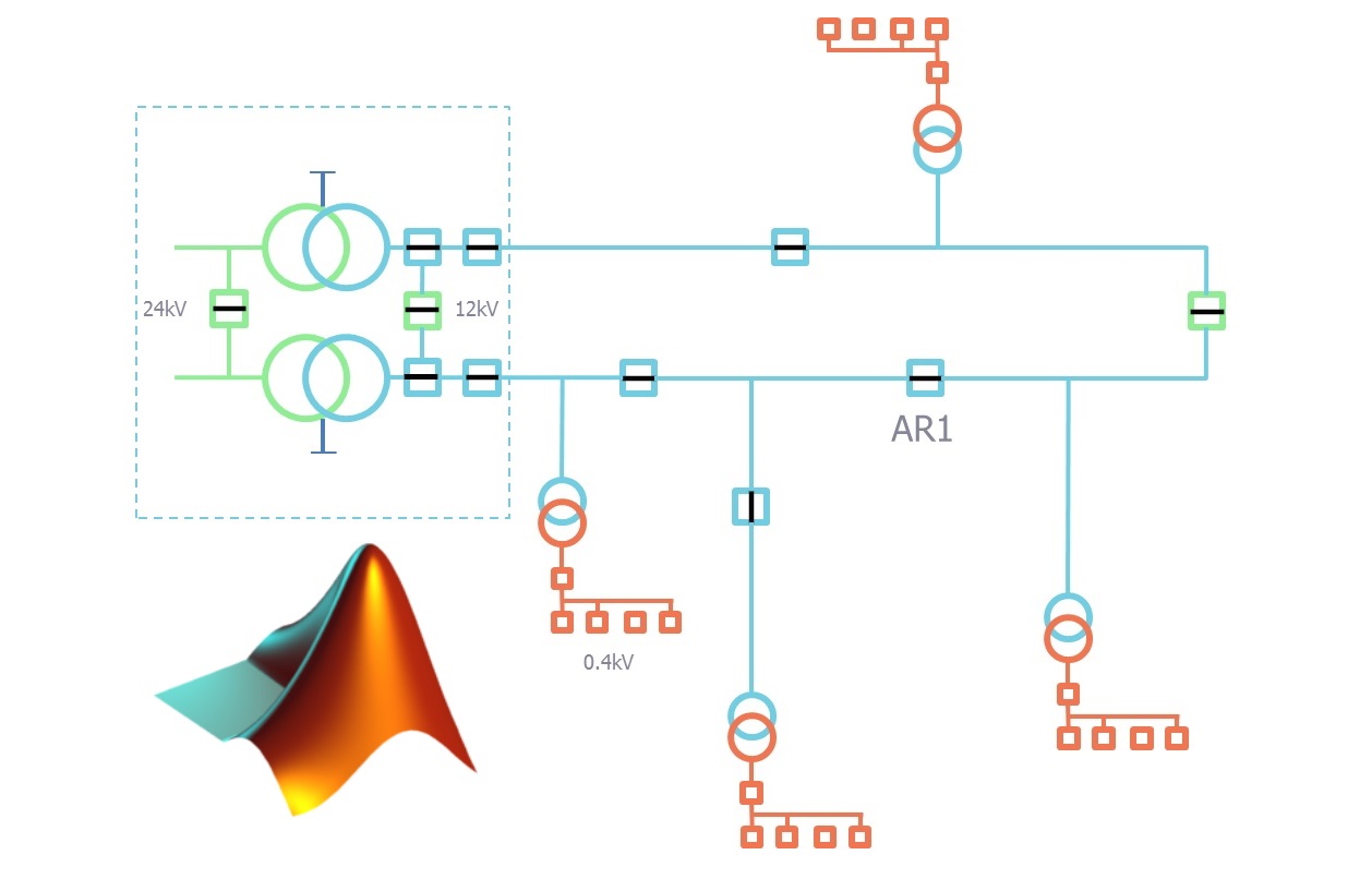
پخش بار نیوتن رافسون در متلب — از صفر تا صد

۱۳۸۲ بازدید
آخرین به‌روزرسانی: ۱۷ اردیبهشت ۱۴۰۲
زمان مطالعه: ۱۴ دقیقه
پخش بار نیوتن رافسون در متلب — از صفر تا صد

در آموزش‌های پیشین مجله فرادرس، با مفاهیم و معادلات پخش بار آشنا شدیم. همچنین روش‌های پخش بار نیوتن رافسون و گوس سایدل را به طور مفصل شرح دادیم. در این آموزش، برنامه‌ پخش بار نیوتن رافسون در متلب را ارائه خواهیم‌ کرد.

قبل از بررسی برنامه‌های متلب، پیشنهاد می‌کنیم آموزش‌های «پخش بار در سیستم قدرت» و «پخش بار نیوتن رافسون» را مطالعه کنید.

در ادامه، خلاصه‌ای از مراحل روش نیوتن رافسون را بیان می‌کنیم.

خلاصه روش نیوتن رافسون

جریان تزریقی هر باس با فرمول زیر محاسبه می‌شود:

$$ \large I _ { i } = \sum _ { j = 1 } ^ { n } Y _ { i j } V _ { j } = \sum _ { j = 1 } ^ { n } \left| Y _ { i j } \right| \left| V _ { j } \right| < \theta _ { i j } + \delta _ { j } $$

با استفاده از این جریان، می‌توانیم معادلات پخش توان‌های اکتیو و راکتیو را بنویسیم:

$$ \large \begin {array} {l} { P _ { i } ^ { [ k] } = \sum _ { j = 1 } ^ { n } \left| V _ { i }^ { [ k ] } \right| \left| V _ { j } ^ { [ k ] } \right| \left| Y _ { i j } \right| \cos \left( \theta _ { i j } - \delta _ { i } ^ { [ k ] } + \delta _ { j } ^ { [ k ] } \right) } \\ { Q _ { i } ^ { [ k ] } = -\sum _ { i = 1 } ^{ n } \left| V _ { i } ^ { [ k ] } \right| \left| V _ { j } ^ { [k ] } \right| \left| Y _ { i j } \right| \sin \left( \theta _ { i j } -\delta _ { i } ^ { [ k ] } + \delta _ { j } ^ { [ k ] } \right ) } \end {array} $$

در نتیجه، با مسئله به فرم $$ f ( x ) = b $$ مواجه خواهیم بود:

$$ \large x ^ { [ k ] } = \left[ \begin {array} {c} { \delta ^ { [ k ] } } \\ { V ^ { [ k ] } } \end {array} \right] \quad f \left ( x ^ { [ k ] } \right) = \left[ \begin {array} {c} { P _ { i n j } \left( x ^ { [ k ] } \right) } \\ { Q _ { i n j } \left( x ^ { [ k ] } \right ) } \end {array} \right] $$

در روش نیوتن رافسون، یک حدس اولیه به صورت زیر داریم:

حدس اولیه $$ x _ { solution} $$ $$ \large x ^ {[0]} = $$          $$ \large c = f ( x _ {solution} )$$

با استفاده از این حدس اولیه، می‌توانیم از خطا برای محاسبه یک حدس جدید استفاده کنیم:

$$ \large x ^ { [ k + 1 ] } = x ^ { [ k ] } + \frac { c - f \left ( x ^ { [ k ] } \right ) } { \left ( d f \left ( x ^ { [ k ] } \right ) / d x \right ) } $$

مخرج کسر، ژاکوبی است و داریم:

$$ \large d f ( x ) / d t \; \; \; \; \Rightarrow \; \; \; \; \left[ \begin {array} {c} { \Delta P } \\ { \Delta Q } \end {array} \right] = \left[ \begin {array} {cc} { \partial P / \partial \delta } & { \partial P / \partial | V | } \\ { \partial Q / \partial \delta } & { \partial Q / \partial | V | } \end {array} \right] \left[ \begin {array} {c} { \Delta \delta } \\ { \Delta | V | } \end {array} \right] $$

الگوریتم پخش بار نیوتن رافسون به طور خلاصه مطابق شکل زیر است.

پخش بار نیوتن رافسون در متلب

برنامه پخش بار نیوتن رافسون در متلب

برنامه اصلی مربوط به پخش بار نیوتن رافسون powerFlow.m است که در ادامه آورده شده است. قبل از اجرای این برنامه مطمئن شوید فایل‌ها و برنامه‌های زیر در پوشه‌ برنامه باشند:

  • فایل BusInputData.csv به عنوان اطلاعات سیستم
  • تابع createYbus.m برای تشکیل Ybus از روی فایل اطلاعات BusInputData.csv
  • تابع data2bus.m برای ذخیره اطلاعات باس در ساختار جدید برای محاسبات
  • تابع findJacob.m برای پیدا کردن ژاکوبی
  • تابع sparseAdd.m که در Ybus مورد استفاده قرار می‌گیرد.
  • تابع calcPQ.m که محاسبات P و Q‌ را انجام می‌دهد.

برنامه‌های فوق را می‌توانید از این لینک [+] دانلود کنید.

درادامه، کد مربوط به هریک از توابع و برنامه‌ها ارائه شده است.

اطلاعات سیستم

فایل ورودی حاوی اطلاعات سیستم BusInputData.csv است که از این لینک [+] قابل دریافت است.

پخش بار نیوتن رافسون

برنامه اصلی پخش بار نیوتن رافسون با عنوان powerFlow.m به صورت زیر است:

1%% POWER FLOW ANALYSIS 
2
3% THIS CODE IS ANALYSES THE COMPLEX POWER FLOW FOR A NETWORK
4
5%Files needed in directory are:
6% BusInputData.csv
7% createYbus.m -forms Ybus from busInputData
8% data2bus.m - stores bus data in new structure for calcs
9% findJacob.m - finds jacobian
10% sparseAdd.m - used in Ybus
11% calcPQ.m - calculations PQ injections using calculated node V and Th
12
13% CODE BY CHRIS MUTZEL
14% CHRIS.MUTZEL@GMAIL.COM
15
16% EE197 - POWER SYSTEMS ANALYSIS
17% PROFESSOR A. STANKOVIC
18% DEPEARTMENT OF ELECTRICAL AND COMPUTER ENGINEERING
19% TUFTS UNIVERSITY, MEDFORD, MA
20
21% DECEMEBER 21TH, 2011
22
23
24clc
25clear
26format short  % keep output to 4 decimal places
27disp('NR Power Flow')
28disp('Code by Chris Mutzel')
29disp('chris.mutze@gmail.com')
30Ttotal = tic;
31
32%load Ybus
33[Ybus, data, N, lines] = data2bus(); 
34save Ybus;
35
36%Create new storage for bustype, P, Q, V, theta
37busData = zeros(N,5);           
38for n=1:N    %populate dataBus
39    busData(data(n,1),1) = data(n,3);                   % bus type
40    busData(data(n,1),2) = (data(n,8) - data(n,6))/100; % Pspec [MW]
41    busData(data(n,1),3) = (data(n,9) - data(n,7))/100; % Qspec [MVAR]
42    busData(data(n,1),4) = data(n,4); % V 
43end                                 
44disp(' '); disp('Specified Injections'); disp('    #         Pspec     Qspec');
45disp([(1:N)' busData(:,2) busData(:,3)])
46busData(1,4) = 1.0; %Slack voltage is one, angle zero
47
48numPV=0;
49for i = 1:N  %find number of each bus type
50   if (busData(i,1) == 2)
51      numPV = numPV + 1; %m
52   end
53end
54m = numPV; % N-m-1 are PQ buses
55
56%Intialize N-R Variables
57ep  = .00000001;                %stopping criteria for bus power mismatches
58STOP = 0;                   %set to one when all deltaPQ < ep
59 
60X = [zeros(N-1,1); 1*ones(N-m-1,1)];    %flat start
61deltaPQ = zeros(2*N-m-2,1);             %Mismatch vector
62j = 0;                                  %iteration count
63
64Traph = tic;                       %Start Timer
65while STOP == 0;
66    if j == 0;
67        disp('######################################################')
68        disp('Begin Newton Raphson')
69        disp('Flat Start->')
70        X
71    end
72    
73  
74    itNum = int2str(j + 1); 
75    disp('######################################################')
76    disp(' '); disp(strcat('Begin Iteration: ',itNum)); disp(' ')
77    
78    % Update V in dataBus for all PQ , use voltages from here for PQcalc
79    c = 1;
80    for n=1:N
81        if busData(n,1) == 0; % if the bus is a PQ bus
82           busData(n,4) = X(N+c-1); % store its V along with knowns for calc
83        c = c+1;
84        end
85    end
86    
87    %Update thetaBus for all PQ, use for PQcalc
88     c = 1;
89     for n=1:N
90         if n == 1;
91            busData(n,5) = 0;
92         end
93         if (busData(n,1) == 2 || busData(n,1) == 0);
94            busData(n,5) = X(c); 
95         c = c+1;
96         end
97         
98     end
99         
100    % ###################################################### 
101    %Calculate PQcalc based on V and theta
102    [Pcalc, Qcalc] = calcPQ(Ybus, busData, N);
103    %disp('    #      Pspec    Qspec')
104    %disp([(1:N)' busData(:,2) busData(:,3)])
105    %disp('    #      Pcalc     Qcalc')
106    %disp([(1:N)' Pcalc Qcalc])
107   
108    % ######################################################
109    %Calculate bus power mismatches
110    
111    %P
112    deltaPQ(1:N-1,1) = busData(2:N, 2) - Pcalc(2:N,1);
113    
114    %Q
115    bc = 0; %counter for index in delta PQ
116    for n=1:N
117        if (busData(n,1) == 0) % only for PQ buses
118            bc = bc + 1;
119            deltaPQ(N+bc-1,1) = busData(n,3) - Qcalc(n,1); 
120        end
121    end
122    %clear bc
123    %disp('Mismatch vector =')
124    %disp(deltaPQ)
125    
126    % ######################################################
127    % Check for convergence
128    error = norm(deltaPQ,2);
129    disp('Error, given by 2-norm of Mismatch vector')
130    disp(error)
131          
132    if (error < ep);
133        STOP = 1;
134        disp('Power Flow Calculation stopped')
135        disp('Error Threshold Reached')
136        disp(' ')
137    end
138    
139    % ######################################################
140    % New iteration if error over threshold
141    if STOP==0;
142        
143        %Find new Jacobian
144        %if j <= 2;
145            Jacob = findJacob(Ybus, Pcalc, Qcalc, busData, N, m);
146        %end
147            
148    % Solve the mismatch equations
149    % Invert the Jacobian
150        invJ = inv(Jacob);
151    % Solve for deltaX 
152        dX = invJ*deltaPQ;
153        
154    %Update Theta and V    
155        X = X + dX;
156    end
157    j = j+1;
158    %if (STOP == 0)
159    %    disp('    #         V       Theta')
160    %    disp([(1:N)' busData(:,4) busData(:,5)*360/(2*pi)])
161    %    disp(strcat('Finished Iteration:', itNum))
162    %end
163    disp(' ')
164    if j >= 10
165        STOP = 1; disp(' ');
166        disp('Power Flow Calculation stopped')
167        disp('Maximum Iterations (10) Reached'); disp(' ')
168    end
169      
170end   %NR iteration
171Traph = toc(Traph); %Stop timer
172
173% ######################################################
174% Newton Raphson Finished
175% Calculate line flows
176Zbus = inv(Ybus);
177lineFlows = [lines zeros(length(lines), 1)];
178for n = 1:length(lineFlows)
179    lineFlows(n,3) =  (exp(1i*angle(Zbus(lineFlows(n,1),lineFlows(n,2))))/abs(Zbus(lineFlows(n,1),lineFlows(n,2))))*...
180        (abs(busData(lineFlows(n,1),4))^2 - abs(busData(lineFlows(n,1),4))*abs(busData(lineFlows(n,2),4))*...
181         exp(1i*(busData(lineFlows(n,1),5) - busData(lineFlows(n,2),5))));      
182end
183
184
185
186Ttotal = toc(Ttotal);
187disp(['Final Solution after ', int2str(j), ' iterations is:'])
188disp('    #         V       Theta')
189disp([(1:N)' busData(:,4) busData(:,5)*360/(2*pi)])
190disp('Line Flows are:')
191disp('  Bus n      to      Bus m              Snm (per unit)')
192disp(lineFlows) 
193disp('Computation Time for NR-iteration was:')
194disp([num2str(Traph), ' seconds'])
195disp('Computation Time for program was:')
196disp([num2str(Ttotal), ' seconds'])

تشکیل ماتریس ادمیتانس شین

تابع CreateYbus.m برای تشکیل ماتریس ادمیتانس شین نوشته شده و برنامه آن به شرح زیر است:

1%% Create Ybus using bus impedance data as input
2
3%% get the data
4clc
5clear
6
7load BusInputData.csv;
8%load testBusData.csv;
9
10data = BusInputData;
11%data = testBusData;
12[a,b] = size(data);
13%data has format: first n rows list the bus numbers in the problem
14% row n+1 holds -999 in first column, marking end input bus #s
15% after -999 is a NaN row, next m entries are impedance data 
16
17% n determines the size of Ybus
18
19%% Read in bus #ing, map to internal numbering
20
21%Find the first row containing -999
22BusIndex = 1;
23stop = 0;
24
25%Find the end of the bus numbering
26while stop == 0
27    if data(BusIndex,1) == -999;
28        stop = 1; 
29    end
30    if (stop == 0);
31        BusIndex = BusIndex + 1;
32    end
33    if BusIndex > a;    
34        stop = 1;
35    end
36end
37
38%Read in the bus numbers and create an internal mapping scheme 
39minBus = min(data(1:BusIndex-1,1));
40maxBus = max(data(1:BusIndex-1,1));
41mapS = minBus - 1; % External number = internal number + mapS
42
43
44
45%%
46clear Ybus;
47%Initialize a sparse matrix element
48Ybus = [maxBus - mapS, maxBus - mapS, 0];
49
50% Find stop point in the data
51stop = 0;
52ConnEnd = BusIndex+1;
53while stop == 0
54    if data(ConnEnd, 1) == -999;
55        stop = 1;
56    end
57    if (stop == 0);
58        ConnEnd = ConnEnd + 1;
59    end
60end
61
62%for each connection, update Ybus
63for n = BusIndex+1:ConnEnd-1
64    NodeA = data(n,1) - mapS; NodeB = data(n,2) - mapS;
65    % Self terms = diagonal elements
66    yab = 1/(data(n,6) + 1i*data(n,7));
67    Ybus = sparseAdd(Ybus, NodeA, NodeA, yab +.5i*data(n,8));
68    Ybus = sparseAdd(Ybus, NodeB, NodeB, yab +.5i*data(n,8));
69    % Off diagonal terms, only fill the upper diagonal
70    if NodeA > NodeB
71        Ybus = sparseAdd(Ybus, NodeB, NodeA, -yab);
72    else
73        Ybus = sparseAdd(Ybus, NodeA, NodeB, -yab);
74    end
75end
76    
77
78%% Construct the real matrix Ybus
79
80YbusRe = zeros(Ybus(end,1:2));
81
82for m=1:length(Ybus)-1;
83    YbusRe(Ybus(m,1),Ybus(m,2)) = Ybus(m,3);
84    if Ybus(m,1) ~= Ybus(m,2)
85        YbusRe(Ybus(m,2),Ybus(m,1)) = Ybus(m,3);
86    end
87end
88
89YbusRe

برنامه محاسبه P و Q

برنامه محاسبه P و Q، تابعی به نام calcPQ.m است که ورودی‌های آن، Ybus و busData بوده و خروجی‌های Pcalc و Qcalc را نتیجه می‌دهد:

1function [Pcalc,Qcalc] = calcPQ(Ybus, busData, N)
2% Summary: Calculates P and Q injections at each node
3% 
4% Inputs:  
5%   scalar N = numNonSlack is # of non slack busses in the power flow
6%   X is column vector with 1st N - 1  entries for non Slack buses [theta]
7%                           then N - m -1  entries for PQ buses [voltage]
8%
9% Outputs:  
10%   PQ injections at all buses
11
12%Create storage for output
13Pcalc = zeros(N,1); %top row will refer to slack bus
14Qcalc = zeros(N,1);
15
16%P
17for i=1:N
18    for k=1:N
19        Pcalc(i,1) = Pcalc(i,1) + busData(i,4)*busData(k,4)*(...
20            real(Ybus(i,k))*cos(busData(i,5)-busData(k,5)) +...
21            imag(Ybus(i,k))*sin(busData(i,5)-busData(k,5)));
22    end
23end
24
25
26for i=1:N
27    for k=1:N
28        Qcalc(i,1) = Qcalc(i,1) + busData(i,4)*busData(k,4)*(...
29            real(Ybus(i,k))*sin(busData(i,5)-busData(k,5)) -...
30            imag(Ybus(i,k))*cos(busData(i,5)-busData(k,5)));
31    end
32end
33
34end

ذخیره اطلاعات باس‌ها در ساختار جدید

تابع data2bus.m برای ذخیره اطلاعات باس در ساختار جدید نوشته شده و به صورت زیر است:

1function [YbusRe,data,numBus, lines] = data2bus()
2
3load BusInputData.csv;
4%load Test3bus.csv;
5
6data = BusInputData;
7%data = Test3bus;
8[a,b] = size(data);
9%data has format: first n rows list the bus numbers in the problem
10% row n+1 holds -999 in first column, marking end input bus #s
11% after -999 is a NaN row, next m entries are impedance data 
12% n determines the size of Ybus
13
14%Find the first row containing -999
15BusIndex = 1;
16stop = 0;
17
18%Find the end of the bus numbering
19while stop == 0
20    if data(BusIndex,1) == -999;
21        stop = 1; 
22    end
23    if (stop == 0);
24        BusIndex = BusIndex + 1;
25    end
26    if BusIndex > a;   % end of file 
27        stop = 1;
28    end
29end
30
31%Read in the bus numbers and create an internal mapping scheme 
32minBus = min(data(1:BusIndex-1,1));
33maxBus = max(data(1:BusIndex-1,1));
34mapS = minBus - 1; % External number = internal number + mapS
35numBus = maxBus - mapS;
36
37clear Ybus;
38%Initialize a sparse matrix element
39Ybus = [maxBus - mapS, maxBus - mapS, 0];
40
41
42% Find stop point in the data
43stop = 0;
44ConnEnd = BusIndex+1;
45while stop == 0
46    if data(ConnEnd, 1) == -999;
47        stop = 1;
48    end
49    if (stop == 0);
50        ConnEnd = ConnEnd + 1;
51    end
52end
53lines = zeros(ConnEnd - BusIndex -1 ,2);
54%for each connection, update Ybus, also store connections
55%lines = zeros(length(BusIndex+1:ConnEnd-1),2);
56for n = BusIndex+1:ConnEnd-1
57    NodeA = data(n,1) - mapS; NodeB = data(n,2) - mapS;
58    lines(n - BusIndex,1) = NodeA;
59    lines(n - BusIndex,2) = NodeB;
60    % Self terms = diagonal elements
61    yab = 1/(data(n,6) + 1i*data(n,7));
62    Ybus = sparseAdd(Ybus, NodeA, NodeA, yab +.5i*data(n,8));
63    Ybus = sparseAdd(Ybus, NodeB, NodeB, yab +.5i*data(n,8));
64    % Off diagonal terms, only fill the upper diagonal
65    if NodeA > NodeB
66        Ybus = sparseAdd(Ybus, NodeB, NodeA, -yab);
67    else
68        Ybus = sparseAdd(Ybus, NodeA, NodeB, -yab);
69    end
70end 
71
72%Construct the real matrix Ybus
73YbusRe = zeros(Ybus(end,1:2));
74
75for m=1:length(Ybus)-1;
76    YbusRe(Ybus(m,1),Ybus(m,2)) = Ybus(m,3);
77    if Ybus(m,1) ~= Ybus(m,2)
78        YbusRe(Ybus(m,2),Ybus(m,1)) = Ybus(m,3);
79    end
80end
81
82
83end

در تابع بالا، از sparseAdd.m استفاده شده که برنامه آن در زیر آمده است:

1function newSparseM = sparseAdd(M, row, col, v)
2%Function for manipulating sparse matrices
3% Input:
4%       M is a sparse matrix object 
5%       row and col are location in a real matrix M to which v should be added
6% Output: 
7%       new sparse matrix element O
8
9% M is ordered by row then by column, third column holds value for row and
10% col.  Last row has holds dimensions of the matrix object
11
12    
13% See if the element exists
14loc = 0;
15found = 0;       % Loc is filled with new position for an element if found  = 0
16c1_index = 1;   % Starting row to check M for existing element
17endloop = 0;    % 
18[a,b] = size(M); % store dimensions of M
19
20while (endloop ~= 1);    
21    if M(c1_index, 1) == row;
22        if M(c1_index, 2) == col;   % the element exists, stores its location
23            loc = c1_index;
24            found = 1;
25            endloop = 1;
26        end
27        if M(c1_index, 2) > col;    % element for same row but higher column   
28            loc = c1_index;
29            found = 0;            
30            endloop = 1;
31        end
32    end
33    
34    if M(c1_index, 1) > row;
35            loc = c1_index;
36            found = 0;
37            endloop = 1; 
38    end
39    c1_index = c1_index + 1;
40    if (c1_index > a)  %Check that we are not out of bounds of the array
41       found = 0;
42       endloop = 1;
43    end
44end
45
46% if it does not exist, create it
47% array has same form up to newly added element, then new element, then
48% remaining contents
49if found == 0;
50    newSparseM = [M(1:loc-1,:); [row, col, v]; M(loc:end,:)];
51end
52
53%If does exist, v is added to element value
54if found == 1;
55    M(loc,3) = M(loc,3) + v;
56    newSparseM = M;
57end
58
59%insert code here to delete row if value is now zero, not important for
60%Ybus since all values remain non-zero once created.
61end

محاسبه ژاکوبی

تابع محاسبه ماتریس ژاکوبی در findjacob.m نوشته شده و برنامه آن به صورت زیر است:

1function [newJacob] = findJacob2(Ybus,Pcalc, Qcalc, busData, N, m)
2% Summary: Finds the Jacobian for the power flow problem given
3%
4% Inputs:
5%   scalar N = numNonSlack is # of non slack busses in the power flow
6%   X is column vector with 1st N entries theta for non Slack buses
7%                           then N entries V for non Slack buses
8%
9% Outputs:
10%   Jacob 
11
12%Create storage for output
13%square matrix with n = N-1 + N - m - 1
14Jacob = zeros(2*N,2*N);
15
16
17sizeJ = 2*N;
18
19for Jr=1:2
20    for Jc=1:2
21        
22        %J11
23        if (Jr == 1 && Jc == 1)
24            for SJr=1:N
25                
26                for SJc=1:N
27                   
28                    if (SJr == SJc) % diagonal elements 
29                        Jacob(SJr,SJr) = -Qcalc(SJc,1) - imag(Ybus(SJc,SJc))*abs(busData(SJc,4))^2;
30                                
31                    else            % off-diagonal elements
32                        Jacob(SJr, SJc) = abs(busData(SJr,4))*abs(busData(SJc,4))*(...
33                            real(Ybus(SJr,SJc))*sin(busData(SJr,5)-busData(SJc,5))-...
34                            imag(Ybus(SJr,SJc))*cos(busData(SJr,5)-busData(SJc,5)));
35                        
36                    end
37                end
38            end
39            
40        end
41        
42        %J12
43        if (Jr == 1 && Jc == 2)
44            for SJr=1:N
45                for SJc=1:N
46                    if SJr == SJc % diagonal elements
47                        Jacob(SJr, N + SJc) = Pcalc(SJc)/abs(busData(SJc,4)) +...
48                            real(Ybus(SJc,SJc))*abs(busData(SJc,4));
49                    else          % off-diagaonal elements
50                        Jacob(SJr, N + SJc) = abs(busData(SJr,4))*(...
51                            real(Ybus(SJr, SJc))*cos(busData(SJr,5)-busData(SJc, 5))+...
52                            imag(Ybus(SJr, SJc))*sin(busData(SJr,5)-busData(SJc, 5)));
53                    end
54                end
55            end
56        end
57        
58        
59        %J21
60        if (Jr == 2 && Jc == 1)
61            for SJr=1:N
62                for SJc=1:N
63                    if SJr == SJc % diagonal elements
64                        Jacob(N + SJr, SJc) = Pcalc(SJc) - real(Ybus(SJc, SJc))*abs(busData(SJc, 4))^2;
65                    else          % off-diagonal elements
66                        Jacob(N + SJr, SJc) = -abs(busData(SJr,4))*abs(busData(SJc,4))*(...
67                            real(Ybus(SJr, SJc))*cos(busData(SJr,5) - busData(SJc,5)) +... 
68                            imag(Ybus(SJr, SJc))*sin(busData(SJr,5) - busData(SJc,5)));
69                    end
70                end
71            end
72        end
73        
74        %J22
75        if (Jr == 2 && Jc == 2)
76            for SJr=1:N
77                for SJc=1:N
78                    if SJr == SJc % diagonal elements
79                        Jacob(N + SJr, N +  SJc) = Qcalc(SJc,1)/abs(busData(SJc,4)) - ...
80                            imag(Ybus(SJc, SJc))*abs(busData(SJc,4));
81                    else          %off-diagonal elements
82                        Jacob(N + SJr, N +  SJc) = abs(busData(SJr, 4))*(...
83                            real(Ybus(SJr, SJc))*sin(busData(SJr,5)-busData(SJc,5))-...
84                            imag(Ybus(SJr, SJc))*cos(busData(SJr,5)-busData(SJc,5)));
85                            
86                    end
87                end
88            end
89        end
90        
91    end
92end
93
94% ######################################################
95%Just found the Jacob for all buses, all only for PQ + PV, PV
96newJacob = zeros(2*N-m-2,2*N-m-2);
97
98%J11
99for c = 2:N
100    newJacob(1:N-1,c-1) = Jacob(2:N, c);
101end
102
103%J12
104a=0;
105for b = 1:N
106    if (busData(b,1) == 0)
107        a = a + 1;
108        newJacob(1:N-1, N-1+a) = Jacob(2:N,b+N);
109    end
110end
111
112%J21
113a=0;
114for b=1:N
115    if (busData(b,1) == 0)
116        a = a + 1;
117        newJacob(N-1+a, 1:N-1) = Jacob(b+N, 2:N);
118    end
119end
120
121%J22
122%nest for loops do same thing as above
123
124a=0;
125for b=1:N
126    if (busData(b,1) == 0)
127        a=a+1;
128        c=0;
129        for d=1:N
130            if (busData(d,1) == 0)
131                c=c+1;
132                newJacob(N-1+a, N-1+c) = Jacob(b+N,d+N);
133            end
134        end
135    end
136end
137end

نتیجه اجرای برنامه

اگر برنامه فوق را اجرا کنیم، نتیجه آن به صورت زیر خواهد بود:‌

NR Power Flow
Code by Chris Mutzel
chris.mutze@gmail.com

Specified Injections
# Pspec Qspec
1.0000 2.9750 0.1420
2.0000 0.1830 0.3730
3.0000 -0.0240 -0.0120
4.0000 -0.0760 -0.0160
5.0000 -0.9420 0.2100
6.0000 0 0
7.0000 -0.2280 -0.1090
8.0000 -0.3000 0.1000
9.0000 0 0
10.0000 -0.0580 -0.0200
11.0000 0 0.2400
12.0000 -0.1120 -0.0750
13.0000 0 0.2400
14.0000 -0.0620 -0.0160
15.0000 -0.0820 -0.0250
16.0000 -0.0350 -0.0180
17.0000 -0.0900 -0.0580
18.0000 -0.0320 -0.0090
19.0000 -0.0950 -0.0340
20.0000 -0.0220 -0.0070
21.0000 -0.1750 -0.1120
22.0000 -0.2000 -0.1000
23.0000 -0.1320 -0.1160
24.0000 -0.0870 -0.0670
25.0000 0 0
26.0000 -0.0350 -0.0230
27.0000 0 0
28.0000 0 0
29.0000 -0.0240 -0.0090
30.0000 -0.1060 -0.0190

######################################################
Begin Newton Raphson
Flat Start->

X =

0
0
0
0
0
0
0
0
0
0
0
0
0
0
0
0
0
0
0
0
0
0
0
0
0
0
0
0
0
1
1
1
1
1
1
1
1
1
1
1
1
1
1
1
1
1
1
1
1
1
1
1
1

######################################################

Begin Iteration:1

Error, given by 2-norm of Mismatch vector
1.4031


######################################################

Begin Iteration:2

Error, given by 2-norm of Mismatch vector
0.1984


######################################################

Begin Iteration:3

Error, given by 2-norm of Mismatch vector
0.0022


######################################################

Begin Iteration:4

Error, given by 2-norm of Mismatch vector
7.0148e-07


######################################################

Begin Iteration:5

Error, given by 2-norm of Mismatch vector
1.4676e-13

Power Flow Calculation stopped
Error Threshold Reached


Final Solution after 5 iterations is:
# V Theta
1.0000 1.0000 0
2.0000 1.0431 -7.7207
3.0000 0.9976 -10.0036
4.0000 0.9985 -12.2845
5.0000 1.0099 -17.0839
6.0000 1.0011 -14.3498
7.0000 0.9969 -16.0041
8.0000 1.0099 -15.2790
9.0000 1.0069 -18.8849
10.0000 0.9727 -21.3515
11.0000 1.0821 -18.8849
12.0000 1.0094 -20.3683
13.0000 1.0709 -20.3683
14.0000 0.9858 -21.5250
15.0000 0.9722 -21.6170
16.0000 0.9854 -21.0250
17.0000 0.9714 -21.5128
18.0000 0.9594 -22.3195
19.0000 0.9551 -22.5191
20.0000 0.9587 -22.2919
21.0000 0.9492 -22.2157
22.0000 0.9466 -22.3079
23.0000 0.9323 -22.4806
24.0000 0.9316 -22.3575
25.0000 0.9459 -21.3307
26.0000 0.9268 -21.8175
27.0000 0.9639 -20.3923
28.0000 0.9971 -15.1012
29.0000 0.9427 -21.7819
30.0000 0.9305 -22.7836

Line Flows are:
Bus n to Bus m Snm (per unit)
30.0000 + 0.0000i 29.0000 + 0.0000i 0.0057 + 0.0047i
29.0000 + 0.0000i 27.0000 + 0.0000i 0.0079 + 0.0074i
30.0000 + 0.0000i 27.0000 + 0.0000i 0.0135 + 0.0114i
27.0000 + 0.0000i 25.0000 + 0.0000i -0.0052 - 0.0063i
25.0000 + 0.0000i 26.0000 + 0.0000i -0.0025 - 0.0068i
24.0000 + 0.0000i 25.0000 + 0.0000i 0.0054 + 0.0046i
24.0000 + 0.0000i 23.0000 + 0.0000i -0.0007 + 0.0002i
14.0000 + 0.0000i 15.0000 + 0.0000i -0.0005 - 0.0047i
15.0000 + 0.0000i 18.0000 + 0.0000i -0.0039 - 0.0044i
18.0000 + 0.0000i 19.0000 + 0.0000i -0.0011 - 0.0015i
19.0000 + 0.0000i 20.0000 + 0.0000i 0.0013 + 0.0012i
12.0000 + 0.0000i 16.0000 + 0.0000i -0.0039 - 0.0084i
17.0000 + 0.0000i 10.0000 + 0.0000i 0.0009 + 0.0005i
22.0000 + 0.0000i 21.0000 + 0.0000i 0.0005 + 0.0009i
21.0000 + 0.0000i 10.0000 + 0.0000i 0.0048 + 0.0077i
22.0000 + 0.0000i 10.0000 + 0.0000i 0.0053 + 0.0085i
12.0000 + 0.0000i 13.0000 + 0.0000i -0.0002 + 0.0217i
12.0000 + 0.0000i 4.0000 + 0.0000i 0.0469 - 0.0069i
2.0000 + 0.0000i 4.0000 + 0.0000i -0.0272 - 0.0163i
10.0000 + 0.0000i 9.0000 + 0.0000i 0.0143 + 0.0111i
9.0000 + 0.0000i 11.0000 + 0.0000i -0.0001 + 0.0262i
9.0000 + 0.0000i 6.0000 + 0.0000i 0.0264 - 0.0029i
10.0000 + 0.0000i 6.0000 + 0.0000i 0.0393 + 0.0068i
28.0000 + 0.0000i 6.0000 + 0.0000i 0.0043 + 0.0013i
28.0000 + 0.0000i 8.0000 + 0.0000i -0.0010 + 0.0042i
6.0000 + 0.0000i 8.0000 + 0.0000i -0.0054 + 0.0028i
6.0000 + 0.0000i 7.0000 + 0.0000i -0.0095 - 0.0016i
6.0000 + 0.0000i 2.0000 + 0.0000i 0.0395 + 0.0114i
7.0000 + 0.0000i 5.0000 + 0.0000i -0.0063 + 0.0042i
1.0000 + 0.0000i 2.0000 + 0.0000i -0.0463 + 0.0111i
1.0000 + 0.0000i 3.0000 + 0.0000i -0.0570 - 0.0058i
3.0000 + 0.0000i 4.0000 + 0.0000i -0.0131 + 0.0000i
4.0000 + 0.0000i 6.0000 + 0.0000i -0.0119 + 0.0007i
27.0000 + 0.0000i 28.0000 + 0.0000i 0.0295 + 0.0095i
24.0000 + 0.0000i 22.0000 + 0.0000i 0.0002 + 0.0048i
2.0000 + 0.0000i 5.0000 + 0.0000i -0.0563 - 0.0160i
14.0000 + 0.0000i 12.0000 + 0.0000i 0.0069 + 0.0080i
15.0000 + 0.0000i 12.0000 + 0.0000i 0.0073 + 0.0124i
15.0000 + 0.0000i 23.0000 + 0.0000i -0.0046 - 0.0136i
16.0000 + 0.0000i 17.0000 + 0.0000i -0.0028 - 0.0048i
20.0000 + 0.0000i 10.0000 + 0.0000i 0.0052 + 0.0046i

Computation Time for NR-iteration was:
0.28689 seconds
Computation Time for program was:
0.53745 seconds

اگر علاقه‌مند به یادگیری مباحث مشابه مطلب بالا هستید، آموزش‌هایی که در ادامه آمده‌اند نیز به شما پیشنهاد می‌شوند:

^^

بر اساس رای ۱۵ نفر
آیا این مطلب برای شما مفید بود؟
اگر بازخوردی درباره این مطلب دارید یا پرسشی دارید که بدون پاسخ مانده است، آن را از طریق بخش نظرات مطرح کنید.
منابع:
Chris Mutzel
نظر شما چیست؟

نشانی ایمیل شما منتشر نخواهد شد. بخش‌های موردنیاز علامت‌گذاری شده‌اند *