شبیه سازی اینورتر در متلب — به همراه کد

۴۷۶ بازدید
آخرین به‌روزرسانی: ۱۶ اردیبهشت ۱۴۰۲
زمان مطالعه: ۵ دقیقه
شبیه سازی اینورتر در متلب — به همراه کد

اینورتر یکی از انواع مبدل‌های الکترونیک قدرت است که کاربرد زیادی در سیستم‌های فتوولتائیک دارد. همان‌طور که می‌دانیم، برق تولیدی یک سلول خورشیدی، جریان مستقیم است و برای آنکه بتوانیم از آن برای دستگاه‌ها و لوازم استفاده کنیم، باید یک اینورتر DC به AC را به کار بریم. در سیستم‌های فتوولتائیک منفصل از شبکه، اینورتر سیگنال DC را به سیگنال AC تبدیل می‌کند. بنابراین، مدل آن باید با توجه به بازده تبدیلش انتخاب شود. در سیستم‌های متصل به شبکه، اینورترها سیگنال خروجی را با توجه تغییر فرکانس و فاز، با شبکه سنکرون می‌کنند. در این آموزش، برنامه شبیه سازی اینورتر در متلب را ارائه خواهیم کرد.

شکل ۱‎‎ منحنی کارایی اینورتر تجاری را که از دیتاشیت آن به دست آمده نشان می‌دهد. این منحنی، بازده اینورتر را با توجه به توان ورودی و توان نامی آن بیان می‌کند.‎

شکل ۱: ‏‎‏‎‏‎‏منحنی بهره یک اینورتر

منحنی بهره‌وری را می‌توان با تابع توانی زیر توصیف کرد:

‎$$ \large \begin{align*}
‎ ‎\begin {array}‎
‎ \eta = c _ 1 \left( \dfrac { P _ \mathrm { P V } } { P _ { \mathrm { I N V } _ R } } \right) ^ { c _ 2 } + c _ 3 \dfrac { P _ \mathrm { P V } } { P _ { \mathrm { I N V } _ R } } > 0 ‎
‎\end {array}‎
‎\end{align*}‎ $$

که در آن، $$P_\mathrm{PV}$$ و $$P_{\mathrm{INV}_C}$$ به‌ ترتیب توان خروجی ماژول PV و توان نامی اینورتر و $$c_1$$، $$c_2$$ و $$c_3$$ ضرایب مدل هستند. با ابزار برازش متلب می‌توان ضرایب مدل اینورتر را محاسبه کرد. توجه کنید که مدل اینورتر متصل به شبکه کاملاً متفاوت است، زیرا به بررسی مشخصات سیگنال نیاز دارد.
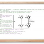
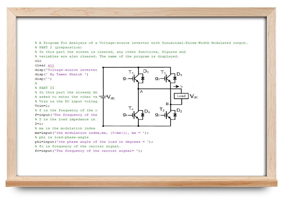
برای مثال، می‌خواهیم برنامه متلب یک اینورتر PWM را با سیگنال خروجی ۵۰ هرتز، شاخص مدولاسیون ۲۰ درصد، فرکانس حامل ۲۰۰ هرتز و زاویه فاز بار ۲۵ درجه بنویسیم. این برنامه به صورت زیر است:

1% A Program For Analysis of a Voltage-source inverter with Sinusoidal-Pulse-Width Modulated output.
2% PART I (preparatihttps://blog.faradars.org/wp-admin/post.php?post=510349&action=edit#on)
3% In this part the screen is cleared, any other functions, figures and
4% variables are also cleared. The name of the program is displayed.
5clc
6clear all
7disp('Voltage-source inverter with Sinusoidal-Pulse Width Modulated output')
8disp(' By Tamer Khatib ')
9disp('')
10%
11% PART II
12% In this part the already known variables are entered, the user is
13% asked to enter the other variables.
14% Vrin is the DC input voltage.
15Vrin=1;
16% f is the frequency of the output voltage waveform.
17f=input('The frequency of the output voltage, f = ');
18% Z is the load impedance in per unit.
19Z=1;
20% ma is the modulation index
21ma=input('the modulation index,ma, (0<ma<1), ma = ');
22% phi is load-phase-angle
23phi=input('the phase angle of the load in degrees = ');
24% fc is frequency of the carrier signal.
25fc=input('The frequency of the carrier signal= ');
26%
27% PART III
28% Calculating load parameters.
29%
30phi=phi*pi/180;
31% R and L are the load resistance and inductance respectively.
32R=Z*cos(phi);
33L=(Z*sin(phi))/(2*pi*f);
34%
35% PART IV
36% Calculating the number of pulses per period,N
37N=fc/f;
38%
39%PART V
40% Building the Sawtooth signal,Vt, the output voltage waveform, Vout,
41% and finding the beginning (alpha) and the end (beta)for each of the output pulses.
42%
43% In each period of the sawtooth, there is one increasing and decreasing part of
44% the sawtooth, thus the period of the output voltage waveform is divided into
45% 2N sub-periods, k is used as a counter of these sub-periods.
46% for calculation purposes each of these sub-periods is divided into 50 points, i.e., the
47% output voltage waveform period is divided into 100N points.
48% j is a counter inside the sub-period
49% i is the generalized time counter
50for k=1:2*N
51for j=1:50
52% finding the generalized time counter
53i=j+(k-1)*50;
54% finding the time step
55wt(i)=i*pi/(N*50);
56%finding the half period of the output voltage.
57if(sin(wt(i)))>0
58hpf=1;
59else
60hpf=-1;
61end
62% calculating the modulating signal.
63ma1(i)=ma*abs(sin(wt(i)));
64% calculating the sawtooth waveform
65if rem(k,2)==0
66Vt(i)=0.02*j;
67if abs(Vt(i)-ma*abs(sin(wt(i))))<=0.011
68m=j;
69beta(fix(k/2)+1)=3.6*((k-1)*50+m)/N;
70else
71j=j;
72end
73else
74Vt(i)=1-0.02*j;
75if abs(Vt(i)-ma*abs(sin(wt(i))))<0.011
76l=j;
77alpha(fix(k/2)+1)=3.6*((k-1)*50+l)/N;
78else
79j=j;
80end
81end
82% calculating the output voltage waveform
83if Vt(i)>ma*abs(sin(wt(i)))
84Vout(i)=0;
85else
86Vout(i)=hpf*Vrin;
87end
88end
89end
90beta(1)=[];
91% PART VI
92% Displaying the beginning (alpha), the end (beta) and the width
93% of each of the output voltage pulses.
94disp(' ')
95disp('......................................................................')
96disp('alpha beta width')
97[alpha' beta' (beta-alpha)']
98% PART VII
99% Plotting the , the triangular carrier signal, Vt,
100% the modulating signal and the output voltage waveform, Vout.
101a=0;
102subplot(2,1,1)
103plot(wt,Vt,wt,ma1,wt,a)
104axis([0,2*pi,-2,2])
105ylabel('Vt, m(pu)');
106subplot(2,1,2)
107plot(wt,Vout,wt,a)
108axis([0,2*pi,-2,2])
109ylabel('Vo(pu)');
110xlabel('Radian');
111% PART VIII
112% Analyzing the output voltage waveform
113% Finding the rms value of the output voltage
114Vo =sqrt(1/(length(Vout))*sum(Vout.^2));
115disp('The rms Value of the output Voltage = ')
116Vo
117% finding the harmonic contents of the output voltage waveform
118y=fft(Vout);
119y(1)=[];
120x=abs(y);
121x=(sqrt(2)/(length(Vout)))*x;
122disp('The rms Value of the output voltage fundamental component = ')
123x(1)
124%
125% Finding the THD of the output voltage
126THDVo = sqrt(Vo^2 -x(1)^2)/x(1);
127%
128% PART IX
129% calculating the output current waveform
130m=R/(2*pi*f*L);
131DT=pi/(N*50);
132C(1)=-10;
133%
134i=100*N+1:2000*N;
135Vout(i)=Vout(i-100*N*fix(i/(100*N))+1);
136%
137for i=2:2000*N;
138C(i)=C(i-1)*exp(-m*DT)+Vout(i-1)/R*(1-exp(-m*DT));
139end
140% PART X
141% Analyzing the output current waveform
142% finding the harmonic contents of the output current waveform
143for j4=1:100*N
144CO(j4)=C(j4+1900*N);
145CO2= fft(CO);
146CO2(1)=[];
147COX=abs(CO2);
148COX=(sqrt(2)/(100*N))*COX;
149end
150% Finding the RMS value of the output current.
151CORMS = sqrt(sum(CO.^2)/(length(CO)));
152disp(' The RMS value of the load current =')
153CORMS
154%Finding the THD for the output current
155THDIo = sqrt(CORMS^2-COX(1)^2)/COX(1);
156% PART XI
157% Finding the supply current waveform
158for j2=1900*N+1:2000*N
159if Vout(j2)~=0
160CS(j2)=abs(C(j2));
161else
162CS(j2)=0;
163end
164end
165% PART XII
166% Analyzing the supply current waveform
167%
168% Supply current waveform and its average value
169for j3=1:100*N
170CS1(j3)=abs(CS(j3+1900*N));
171end
172CSRMS= sqrt(sum(CS1.^2)/(length(CS1)));
173disp('The RMS value of the supply current is')
174CSRMS
175CSAV= (sum(CS1)/(length(CS1)));
176disp('The Average value of the supply current is')
177CSAV
178% Finding the Fourier analysis of the supply current waveform
179CS2= fft(CS1);
180CS2(1)=[];
181CSX=abs(CS2);
182CSX=(sqrt(2)/(100*N))*CSX;
183% PART XIII
184% Displaying the calculated parameters.
185disp(' Performance parameters are')
186THDVo
187THDIo
188a=0;
189%PART XIV
190% Opening a new figure window for plotting of
191% the output voltage, output current, supply current and the harmonic
192% contents of these values
193figure(2)
194subplot(3,2,1)
195plot(wt,Vout(1:100*N),wt,a);
196title('');
197axis([0,2*pi,-1.5,1.5]);
198ylabel('Vo(pu)');
199subplot(3,2,2)
200plot(x(1:100))
201title('');
202axis([0,100,0,0.8]);
203subplot(3,2,3)
204plot(wt,C(1900*N+1:2000*N),wt,a);
205title('');
206axis([0,2*pi,-1.5,1.5]);
207ylabel('Io(pu)');
208subplot(3,2,4)
209plot(COX(1:100))
210title('');
211axis([0,100,0,0.8]);
212ylabel('Ion(pu)');
213subplot(3,2,5)
214plot(wt,CS(1900*N+1:2000*N),wt,a);
215axis([0,2*pi,-1.5,1.5]);
216ylabel('Is(pu)');
217xlabel('Radian');
218subplot(3,2,6)
219plot(CSX(1:100))
220hold
221plot(CSAV,'*')
222text(5,CSAV,'Average valu')
223title('');
224axis([0,100,0,0.8]);
225ylabel('Isn(pu)');
226xlabel('Harmonic Order');

اگر این برنامه را اجرا کنیم، از ما خواسته می‌شود که اطلاعات زیر را وارد کنیم‌. این اطلاعات را با توجه به اعداد مذکور بالا وارد می‌کنیم:

Voltage-source inverter with Sinusoidal-Pulse Width Modulated output
By Tamer Khatib 
The frequency of the output voltage, f = 50
the modulation index,ma, (0<ma<1), ma = 0.2
the phase angle of the load in degrees = 25
The frequency of the carrier signal= 200

در نتیجه، خروجی برنامه به صورت زیر خواهد بود:

......................................................................
alpha beta width

ans =

   39.6000   52.2000   12.6000
  127.8000  140.4000   12.6000
  219.6000  232.2000   12.6000
  307.8000  320.4000   12.6000

The rms Value of the output Voltage = 

Vo =

    0.3742

The rms Value of the output voltage fundamental component = 

ans =

    0.1408

 The RMS value of the load current =

CORMS =

    0.1859

The RMS value of the supply current is

CSRMS =

    0.0906

The Average value of the supply current is

CSAV =

    0.0295

 Performance parameters are

THDVo =

    2.4618


THDIo =

    0.8624

Current plot held

شکل ۲، ولتاژ خروجی پریونیت اینورتر را نشان می‌دهد.

شکل ۲: خر.جی مدل اینورتر 
شکل ۲: خروجی مدل اینورتر

شکل ۳ نیز ولتاژ و جریان را نشان می‌دهد.

شکل ۳: خروجی اینورتر 
شکل ۳: خروجی اینورتر

اگر این مطلب برای شما مفید بوده و علاقه‌مند به یادگیری مباحث مشابه هستید، آموزش‌های زیر را نیز به شما پیشنهاد می‌کنیم:

^^

بر اساس رای ۰ نفر
آیا این مطلب برای شما مفید بود؟
اگر بازخوردی درباره این مطلب دارید یا پرسشی دارید که بدون پاسخ مانده است، آن را از طریق بخش نظرات مطرح کنید.
منابع:
Modeling of Photovoltaic Systems Using MATLAB
نظر شما چیست؟

نشانی ایمیل شما منتشر نخواهد شد. بخش‌های موردنیاز علامت‌گذاری شده‌اند *